P-values are everywhere — in medical trials, economics papers, investing backtests, and credit-risk models — and they’re often misunderstood. A p-value is not the probability that the null hypothesis is true, nor is it a guarantee that a result is practically important. This guide explains what p-values do (and don’t) tell you, how to interpret them alongside effect sizes and confidence intervals, and how to avoid common traps like p-hacking and multiple testing. It reflects the American Statistical Association’s guidance and editorial standards adopted by major journals since 2016–2019.
Key Takeaways
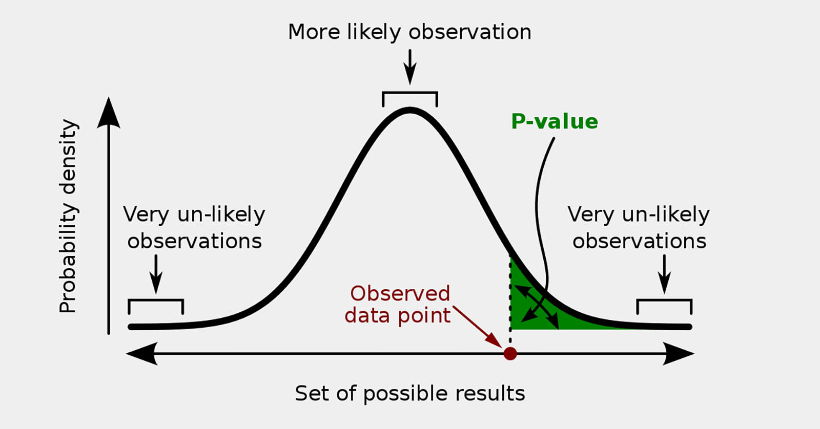
- Definition (correct): The p-value is the probability of obtaining results at least as extreme as those observed, assuming the null hypothesis is true.
- What it is not: It is not the probability the null is true, the probability results are “due to chance,” or a measure of effect size or importance.
- Avoid dichotomies: “Significant” vs. “not significant” at p < 0.05 is a convention, not a law; context, design quality, and prior evidence matter.
- Think in families of evidence: Pair p-values with effect sizes, confidence intervals, statistical power, and (when relevant) multiplicity adjustments.
- Guardrails: Pre-register analyses, resist data dredging, and report all tested hypotheses to curb false positives.
What a P-Value Really Means
Formal definition. The p-value is the probability, under a specified null hypothesis, of observing a test statistic at least as extreme as the one actually observed. In symbols for a right‑tailed test, p = P(T ≥ tobs | H0 is true). For two‑tailed tests, probability mass in both tails is included. This definition matches the NIST Engineering Statistics Handbook and standard statistical texts.
Interpretation. Small p-values indicate that the observed data would be unusual if the null were true; they count as evidence against the null. Large p-values mean the data are compatible with the null but do not prove it. Evidence exists on a continuum; p = 0.049 and p = 0.051 are practically indistinguishable.
Conventional thresholds. Analysts often use 0.10, 0.05, or 0.01 as decision cutoffs. These are historical conventions, not universal rules. The ASA cautions against basing conclusions or policy on a single threshold without considering study design, assumptions, and external evidence.
How to Use P-Values Responsibly (ASA Principles)
The American Statistical Association (ASA) summarized six core principles for interpreting p-values. In brief:
- 1. P-values indicate incompatibility between data and a specified model (usually the null); they are not the probability the model is true.
- 2. Do not base conclusions solely on p-values — always consider effect sizes, uncertainty, design quality, assumptions, and real‑world costs/benefits.
- 3. P-values do not measure the size or importance of an effect or the probability that results were produced by random chance alone.
- 4. Proper inference requires transparency — pre-specification, full reporting, and avoiding selective analysis.
- 5. A p-value does not quantify evidence for a model without context; identical p-values can correspond to different evidential strength.
- 6. P-values can be misused when treated as binary pass/fail metrics; complement them with other approaches.
Since 2019, ASA editors and Nature have urged moving “beyond p < 0.05” toward richer, contextual evidence that emphasizes estimation, transparency, and replicability.
From “Is It Significant?” to “How Big, How Uncertain, and At What Cost?”
Report effect sizes. Always quantify the magnitude of the estimated effect (e.g., mean difference, regression coefficient, odds ratio). A tiny but statistically significant effect may be economically trivial in investing or credit risk once costs and constraints are included.
Show confidence intervals (CIs). CIs display a range of plausible values for the effect under repeated sampling assumptions. Narrow intervals suggest precision; wide intervals signal uncertainty. A result with p = 0.04 but a CI spanning economically negligible values should be treated cautiously.
Check power. Low-powered tests inflate false negatives and, when significant, tend to overstate effect sizes (“winner’s curse”). Prospectively target adequate power; retrospectively interpret marginal p-values with care, especially in small samples.
Consider prior evidence. In domains with many implausible hypotheses (e.g., hundreds of technical trading rules), the prior probability of a true effect may be low; even small p-values can have low positive predictive value without independent replication.
Multiple Testing, P-Hacking, and False Discoveries
Multiplicity. Testing many hypotheses inflates the chance of at least one false positive. If you test 100 rules at α = 0.05, you expect ~5 “significant” hits by chance. Adjustments help control error rates:
- Family-wise error rate (FWER): Bonferroni (divide α by the number of tests), Holm step‑down (more powerful than Bonferroni).
- False discovery rate (FDR): Benjamini–Hochberg (controls expected proportion of false positives among discoveries) — widely used in high‑dimensional settings.
P-hacking/data dredging. Tuning models until something “works” and then reporting only the winner yields biased p-values. Guardrails: pre-registration, holdout sets, out-of-sample tests, and full disclosure of the testing universe.
Regulatory example. In clinical trials, the FDA expects prespecified strategies to address multiplicity across endpoints (e.g., hierarchical testing, Holm, or gatekeeping). Similar discipline helps financial researchers avoid overclaiming.
Practical Reading Guide for Financial and Business Research
- Ask “what was tested?” How many outcomes, subgroups, time windows, or strategies were examined?
- Look for estimation. Are effect sizes and CIs front and center? Are the effects economically material after costs and slippage?
- Scrutinize robustness. Do results replicate in fresh data? Are they sensitive to alternative specifications or small perturbations?
- Mind assumptions. Were distributional assumptions checked (normality, independence, homoskedasticity)? Were nonparametric or robust methods considered?
- Beware thresholding. Claims hinging on p = 0.049 vs. 0.051 deserve skepticism; focus on the weight of evidence.
Worked Mini‑Examples
A strategy shows 12% average annual return vs. 10% for the benchmark over five years. A t‑test yields p = 0.15. This is not strong evidence: under the null of no true edge, results this extreme occur 15% of the time. Conclusion: insufficient evidence; demand longer samples, different markets, or out‑of‑sample tests.
In a default model, “months since last delinquency” has p = 0.002 and an odds ratio of 0.94 per month (95% CI 0.91–0.97). This is both statistically and practically meaningful. Document the effect size, add robustness checks, and validate out of time.
Frequently Asked Questions (FAQs)
Does p = 0.03 mean there is a 97% chance the effect is real?
No. It means that, if the null were true, results this extreme (or more extreme) would occur 3% of the time. It is a statement about data under the null, not about the probability a hypothesis is true.
Is p < 0.05 “proof” of a result?
No. Treat it as one piece of evidence. Consider design quality, assumptions, effect size, uncertainty, costs, and prior evidence. Many journals and the ASA encourage moving beyond binary significant/not‑significant labels.
What should I report besides p-values?
Effect sizes with confidence intervals, protocols and any deviations, all hypotheses tested (or a clear accounting of the family of tests), the analysis code and data (when possible), and sensitivity/robustness checks.
How do one‑tailed and two‑tailed tests change p-values?
One‑tailed tests place all probability mass in a single direction and can yield smaller p-values if the effect is in the predicted direction — but they cannot detect effects in the opposite direction. Use them only when a negative‑direction effect would not change your conclusion or action.
Are Bayesian methods a replacement?
They answer different questions — Bayesian approaches can yield direct probabilities for hypotheses or parameters given priors. Many analysts use both: estimation with intervals plus Bayesian checks when appropriate.
Sources
- American Statistical Association (2016). ASA Statement on P‑Values and Statistical Significance.
- Wasserstein, Schirm & Lazar (2019). Moving to a World Beyond “p < 0.05”. The American Statistician.
- Amrhein, Greenland & McShane (2019). Retire statistical significance. Nature.
- NIST/SEMATECH Engineering Statistics Handbook: Critical values and p-values.
- FDA (2022). Multiple Endpoints in Clinical Trials — Guidance for Industry (multiplicity control).